Plot the Posterior PDFs

You can examine the posterior probability density functions to get a quantitative look at the results of the model fitting process using visualize.posteriorPDF():

import visualize
visualize.posteriorPDF()

This will produce a series of histograms showing the posterior probability distribution functions for every parameter in the model.

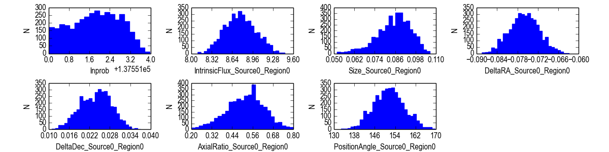
This routine also prints the average and 1-sigma rms uncertainty on each parameter of the model. We can see from the posterior PDF histograms that XMM101 appears to be elongated (axial ratio = 0.52 +/- 0.11) and has a total flux density at 870um of 8.76 +/- 0.24 mJy. It has an effective radius of 0.085 +/- 0.010 arcsec, which translates to a FWHM of 0.2 arcsec. At z=2 (the actual redshift of this object is unknown currently, but the Herschel photometry indicates z~2) this corresponds to a physical size of 1.7 kpc.

You can also see how the posterior PDF of every parameter in the model changes as a function of iteration using visualize.evolvePDF():

visualize.evolvePDF()

This function essentially produces a posteriorPDF every stepsize iterations. The default is stepsize = 50000. You can then view the evolution in the PDF using a viewer application like Preview.